A coupler-based SWR probe radio head for 5 GHz WiFi
Contents
Introduction
On my job of a PC service techie, I'd been wondering for a while,
if it would be possible for me to check the actual properties of some
WiFi antennas that I occasionally homebrew. I don't have a 6GHz vector
analyzer or some such, but I noticed that the HAM's were using various
"coupler heads" to gauge the SWR of their short-wave antennas:
either resistor-based, or more appropriately, actual "directional couplers".
A few PCB-based designs can be found in the sheer stretches of the interwebs.
The basic principle of a "coupled line directional coupler"
is a section of a twin parallel transmission line, where a part
of the EM energy seeps from the master line to the tap line.
Effectively we're trying to achieve some well defined crosstalk here.
The "tap" transmission line should essentially be "just the right
length" for the desired frequency, or at least roughly in the ballpark.
The million dollar question seems to be: what is "just the right length"?
Even uncle Google doesn't have a well argued opinion.
λ/4 sounds like a promising boundary, but in what sense?
Is it the sweet spot, or a snake pit?
Also, while there are simple formulae to calculate a stripline TML
impedance for a single trace, any sort of math to calculate the
coupling (crosstalk) between two parallel TML's is
nearly impossible to find or pretty complex. But you certainly
want the coupling to be "just the right level" as well, right?
Not to siphon too much energy from the master TML, but if OTOH
the output comes out too low, you possibly won't see anything
on the 'scope...
Qucs to shed some light
Quite to my amazement, I discovered that Qucs can actually do
quite a lot for me in this vein :-) For a few months now,
Qucs contains a library of transmission line components,
including a twin-parallel coupled microstrip line :-) Yay!
I noticed voices in the qucs fora, complaining that the TML simulations
were not perfect yet... On the contrary I have to say that Qucs
has worked quite nicely for me on this front.
When I tried some redneck experiments resulting in unexpected outcomes
from Qucs, after some thought I always found out that
Qucs was actually right... This is what simulators are for :-D
In Qucs, I didn't try to combine the RF coupling and transfer simulations
with a rectifying detector (non-linearity). I did actually,
and it didn't come out very well. The RF stuff and near-DC rectification
are probably two very different problem domains... so I just gave up on
the detector in Qucs and focused on simulating the coupled transmission
lines:
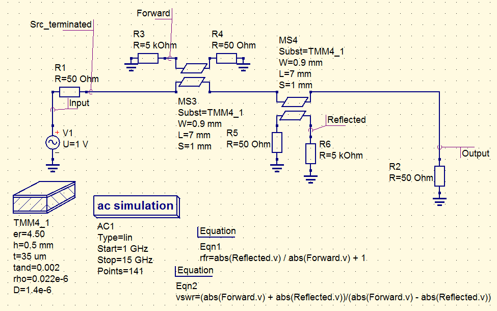
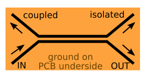
5GHz coupler, as simulated in Qucs
Theoretically, if you can guarantee a proper impedance match
at both ends, a single μstrip "tap line" (double-ended) should be
enough to give you a forward and reflected ports.
One port is "coupled" in the forward direction, and the one
that's "isolated" for the forward wave becomes "coupled"
for the reflected wave (and vice versa).
In reality, it's probably a good idea to have two separate
taps, one each way, to be able to clearly terminate
the isolated end of each tap line.
The detector is a nonlinear pain in the youknowhat.
Moreover, you may want to keep the tap output ports
(sensing points) at a higher-than-matching impedance,
which gives you higher readings on your meter (hopefully
without adverse effects such as reflections on the master
line). If you try to properly terminate the "sensing"
(coupled, hot) end of the tap line, that may feel good,
but the output voltage turns out significantly lower,
and the overall shape of the spectral transfer curve
of the tap remains pretty much unchanged => there's
hardly any point in terminating the hot end of the tap TML.
One thing is for sure (or is it? so they say):
you absolutely MUST terminate the "cold" end of each tap TML
by a matching resistor against the ground plane!
to get a meaningful reading at the "hot" end.
Note that I did not use the Smith chart / energy transfer
/ S-parameters, which comes with its own style of "power sources"
(looks like a voltage source with an integrated series resistor).
Instead, I used a normal AC voltage source, and added a series
resistor of my own (for source termination). Next, I charted some
voltages of interest in a basic V/f chart (Bode magnitude plot).
Initially I walked around the Smith chart because I did not
understand it. Later, after I read some introes into the basic
S-parameter theory and Smith chart wizardry, I concluded that
I was right to do it that way, as the Smith chart wasn't
necessarily very suitable for the display of the information
that I was after. The Smith chart is typically used to display
the reflection coefficient on a particular port, rather than
power transfer between ports (although the
S-parameters for that are certainly available).
To chart the power transfer from the input port to a tap port
sounds like stretching it a little too far :-)
(Perhaps I just should've used the Bode plot to display
the S-parameters. But I'd probably get similar results anyway.)
Anyway - this was the outcome:
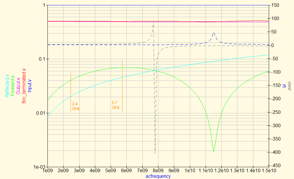
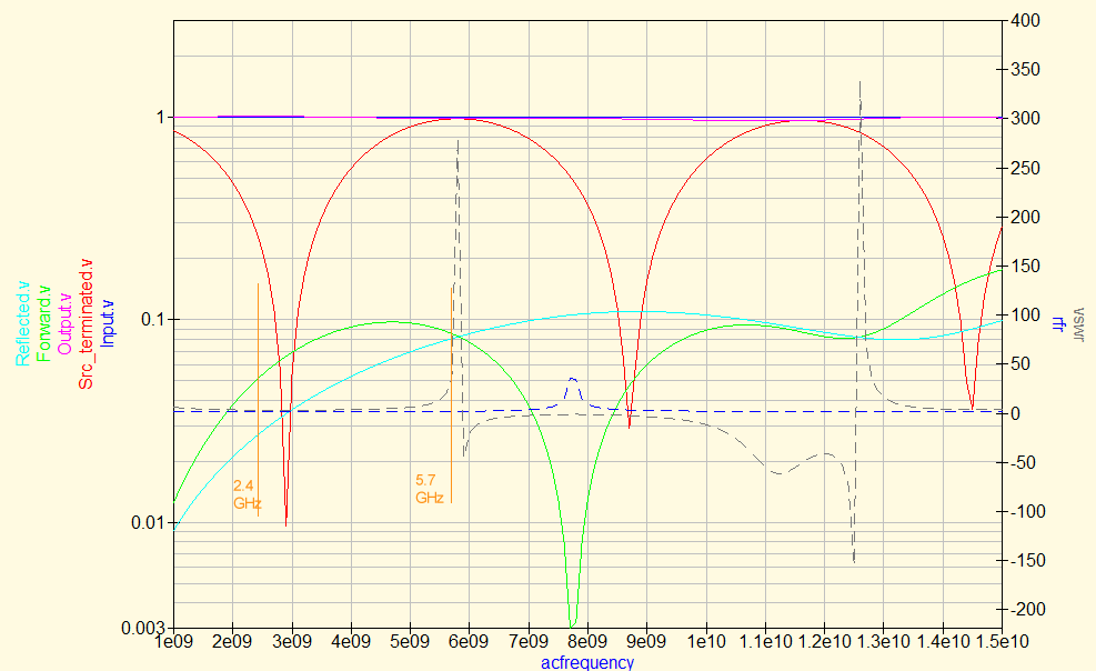
5GHz coupler, Qucs simulation output, output terminated
An important note right here: in this simulation,
the radio head is terminated! I.e., the output
of the master TML can see a perfect impedance-matched load.
Note how curved the voltages are, at the tap outputs!
(see the green and cyan lines.)
I actually tried a few different tap lengths, to see how the
Bode plot changes. The word of mouth was, that λ/4 was a hard
limit, but that the lower end of the useful band was somewhat open.
I was wondering in what way λ/4 was and end, and the plot
seems to give a clear answer. At λ/4, "everything has
gone nuts long ago" :-) See the sharp null on the green line
at about 11.5 GHz ? That looks like a λ/4 corresponding to
just below 7 mm at the speed of light. Or perhaps λ/4 is the
8 GHz "crossing point" of the green vs. cyan lines? Considering the
velocity factor in FR4? 66% looks pretty plausible. Never mind my
crackpot VSWR plot which I left in the sketch just for fun.
Considering the tap signal levels, λ/8 (at velocity 100%)
looks like a plausible tradeoff between sense output signal level,
distinction between forward vs. reflected and generally the desired
sane behavior of the sense signals.
I had the basic TML Z0 calculated ahead of time:
there are formulas in textbooks and calculators on the web,
but there's actually a dedicated calculator tool inside Qucs as well.
So I knew that for a 0.5mm FR4 substrate, I needed about 0.9 mm
trace width.
What I did not know in advance, was the needed spacing
between the main and tap lines in the coupled section. I started out
roughly with some values observed in other people's couplers,
and I kept iterating towards my desired coupling level of about
-20 dB = 1:10th the voltage at the nominal frequency of 5.75 GHz.
The qucs schematic and the PCB layout (below) reflect the spacing
thus inferred, it was about 0.8 to 1 mm if memory serves.
Obviously, I was eager to have Qucs calculate the VSWR for me,
and I tried fumbling for some formulas to calculate VSWR from the
voltages observed on the "forward" and "reflected" taps.
Unfortunately I had to conclude that I was trying to cut too many
corners in one go :-) The voltages on the coupler's outputs
are not directly suitable for SWR calculation.
Quite early on I noticed that although the magnitude plots showed
an absolute value of the voltage, the voltages inside the Qucs engine
are actually complex numbers = with the phase component included.
This dawned on me when my formulas using a simple division (fraction)
resulted in some unexpected curves :-) I was able to correct for this
by using explicit absolute values = the abs() function in my formulas.
But, still the results were not what I expected - and I realized,
that I was using the wrong inputs into the well-known official
VSWR formula. That my voltages followed some logic of their own,
and their relationship to the actual forward vs. reflected
signals on the master TML was not precisely a direct proportion.
Just look at the green and cyan curves - pretty clear, right?
Again the master TML is terminated, hence there should be a strong
forward wave and a zero reflected wave, at any frequency.
If I wanted to "align" the green and cyan lines to that fact,
I would probably need some semi-manual calibration and non-trivial
postprocessing on the tap outputs.
Finally I left the formulas for VSWR and a simple
"reflected to forward ratio" in my Bode plots
for public entertainment :-)
"Okay, but so what use are those curves then?" I can hear you wonder.
"Forward and reflected taps. What use are those signals?"
Apparently the answer is all but simple.
Essentially, as long as the "reflected" sense is noticeably weaker
than the forward signal, you're probably fine, you have a good impedance
match on the output. The forward signal also corresponds to the actual
output power.
If you open the output or short it, the reflected signal should change.
In my case, with the tap lengths as per my design, you get the reflected
signal about as strong as the forward signal. And yes, this corresponds
to an actual perfect reflection, positive or negative.
To shed some more light on the behavior of the two output signals,
let me follow up with two more simulated spectral responses.
You guessed it: open-ended and shorted.
They also chime in on the original topic of "how long should the taps
optimally be", compared to wavelength, and how sensitive the measurements
are to the actual tap length.
5GHz coupler, Qucs simulation output, output open ended
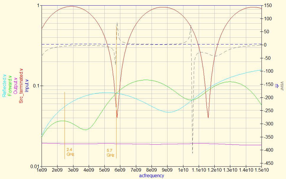
5GHz coupler, Qucs simulation output, output shorted
Note that at 5.7 GHz, my 7mm taps result in a reasonable indication
that the coupler output is shorted or open-ended.
Perhaps more interestingly, note how the shorted or open-ended coupler
behaves at e.g. 2.4 GHz. Based on general popular belief, the coupler
should function in a pretty broad range of frequencies, way down from the
"design nominal frequency", with just the magnitudes of the sense outputs
gradually fading (both at the same time, so the relative information
is still there). See the first "terminated" Bode plot for a likely
source of this belief.
Based on my two simulations (shorted and open), this sounds more like
a "myth just debunked" :-)
At 2.4 GHz, this coupler gives pretty boring magnitudes for
"open ended output", as if nothing happend, as if the main output
was correctly terminated (which is "wrong" WRT our needs) and for
"shorted output", the forward vs. reflected sense output voltages
"swap positions", which is quite amazing to an unprepared
observer :-) I was indeed quite shocked to see this on my 'scope
while trying to watch a WiFi client talk to an AP at 802.11a.
At the time I had no clue what I was looking at (I only did the
open+shorted sims later on). At a first sight, it felt like
I had inadvertently swapped the probes of my 'scope - which I was
pretty sure I did not. I literally felt dizzy :-) Well now I know:
when I tried shorting the output, suddenly the WiFi client lost
the ESSID in the 5 GHz band, and tried probing the 2.4 GHz band
as well = sent a "probe request" frame at full power (this is called
active scanning, useful for AP's with a "hidden ESSID"). Which resulted
in a nice, clean and strong reading on the 'scope, with traces that
"exchanged positions" :-)
In other words / to sum up, the coupler-based measurement head
actually seems to work for a somewhat narrow band of frequencies.
It's not nearly an ideal broadband device.
Perhaps it would be possible to construct a transmission-line
coupler with more broadband properties, using some arcane μstripe
scattering magic... I've tried playing around in Qucs a bit,
but my results only ever got worse than the basic shape presented here :-)
BTW, can you see the "harmonic nulls" on the red curve in the
open/shorted Bode plots? This is the voltage on the output of our generator,
after the series-termination resistor.
I've seen that shape before. On someone's frequency-domain reflectometer
(VNA). The guy immmediately knew "there's a problem somewhere in the cable,
either a short, or a cold joint". That was before I built my own
TDR plug.
Note how straight the red line is on the "terminated" Bode plot.
Sadly, looking at the simulated Bode plots, the coupler attached
to a transmitting wifi radio will only show you two points on the
green and cyan lines :-( You would need at least a wobbler
or a noise source, and a spectrum analyzer, to show you the
full picture.
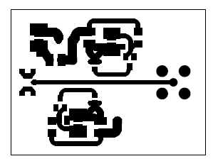
Eagle is my drawing board
Time to take a look at the practical schematic and PCB of my
"coupler-based radio head".
Because my other equipment (oscilloscope, rtl-sdr) is too slow
to capture the WiFi carrier bands, I had to equip my coupler-based
radio head with built-in "envelope detection" = AM demodulation
= RF rectification. Consequently, on my scope I don't see the
WiFi AC carrier, I only see its envelope = signal with a strong
DC component.
There are again two taps / sections, called coupled/isolated
or forward/reverse. In each section, the diode rectifies the
signal to charge a small capacitor. The capacitor effectively
works as a low-pass filter. The trouble is, that the diode
has a forward voltage of about 200-300 mV, which is on par
with the useful signal. To be able to see smaller signals
too, you need to "bias" the diode = pull it slightly open
with a resistor to some DC voltage potential.
For practical reasons, esp. because positive DC voltages
are easily available and the RF signal is referenced to GND,
the easiest way to do the biasing is to connect the
pull-up resistor to the +Vcc rail and have the diode "pull down".
Thus, the resulting "detected" envelope is a negative signal
in the hundreds of millivolts, DC-shifted up by several Volts.
Peaks growing down from +5 V :-)
Where I live, reverse-polarity SMA connectors are somewhat
difficult to come by, especially the PCB-mounted variety.
So I just gutted the angled PCB-mount RPSMA female from the
carcass of an old AP, and I used a U.FL male (the PCB-mount
part, also from the electro junk bin) for the other end
of the coupler. This allows me to test pigtails or bare antennas,
depending on which way I hook up the coupler. The coupler is
otherwise bidirectional, so it doesn't matter which way
I hook it up - only the coupled/isolated taps swap roles
accordingly.
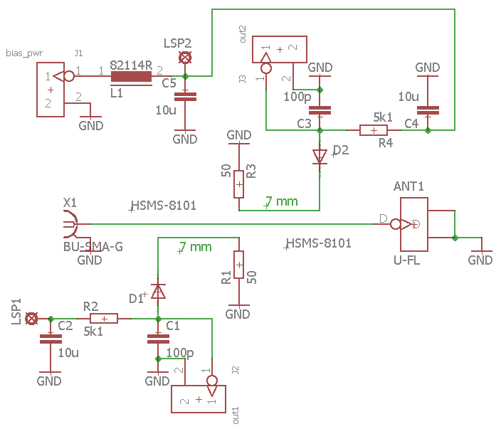
5GHz coupler + detector: a practical schematic
Notes:
For bias power, you can use +5V from e.g. a USB socket.
The diodes used in my schematic, the HSMS-8101, are a fast Schottky,
but nominally a mixer diode, rather than a detector diode.
Its sibling HSMS-2860 would be a nominally more appropriate
part, but it wasn't as easily available to me. Looking at the
I/U curve of both those diodes, the difference is relatively
small, so it probably doesn't matter much. Note that the
2860 has a different pinout than the 8101, but as the cathode
is always at pin 3, the PCB would probably work
without a layout modification.
The pads labeled LSP1 and LSP2 are a wire bridge for the
bias voltage. I wanted to avoid cutting across the GND plane
or routing a power trace all around the signals plane.
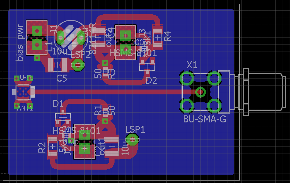
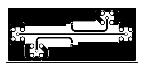
5GHz coupler + detector: my PCB layout
I used 2.5mm dual-pin headers for the outputs and for the bias power input.
And the bias power input choke is again something from trash.
Downloads
Based on my "research into coupler technology", originally done
in the 5 GHz band, I also quickly sketched a simpler coupler
for 1.6 GHz. I had some business to do with the GPS antenna technology,
and I wanted to check some stuff... which ultimately failed due to lack
of a proper signal source (a noise generator for 1.6 GHz is not so
easy to cobble together), but the coupler exists nonetheless,
so I'm including it as a "bonus chapter" :-)
Here are the Qucs data files for both of my couplers.
As for PCB's:
The following pictures are the top layer of my two couplers.
The top layer is where interesting stuff happens.
The bottom layer of my PCB's is equally important,
but boring - it's just a flood-filled ground plane,
providing the GND to the 50 Ohm μstripe transmission lines.
The data files obviously contain both layers (including the bottom layer in PDF).
5 GHz coupler + detector PCB
[Eagle source + PDF]
1.6 GHz coupler (no detector)
[Eagle source + PDF]
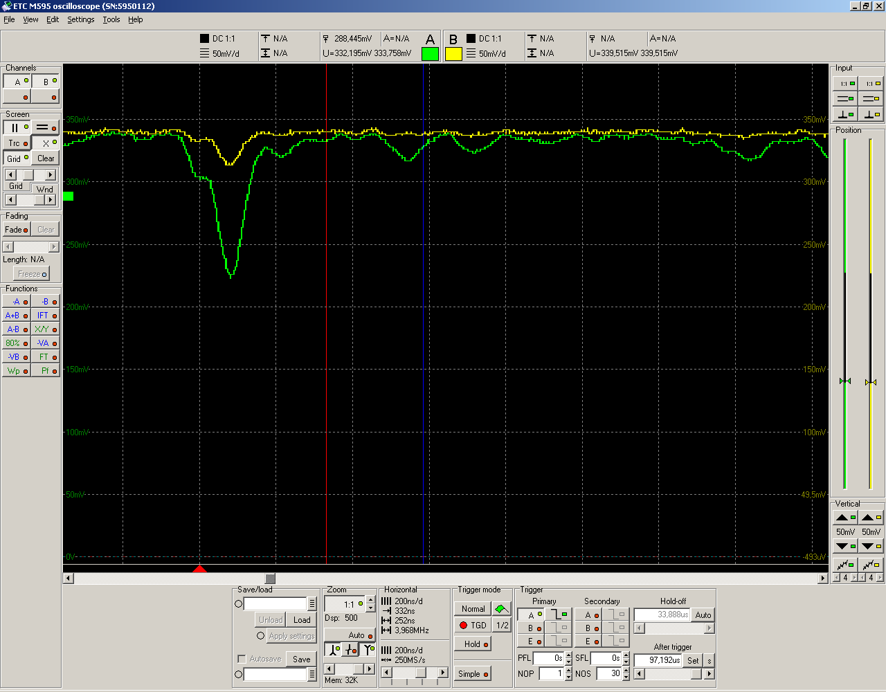
Example measurements
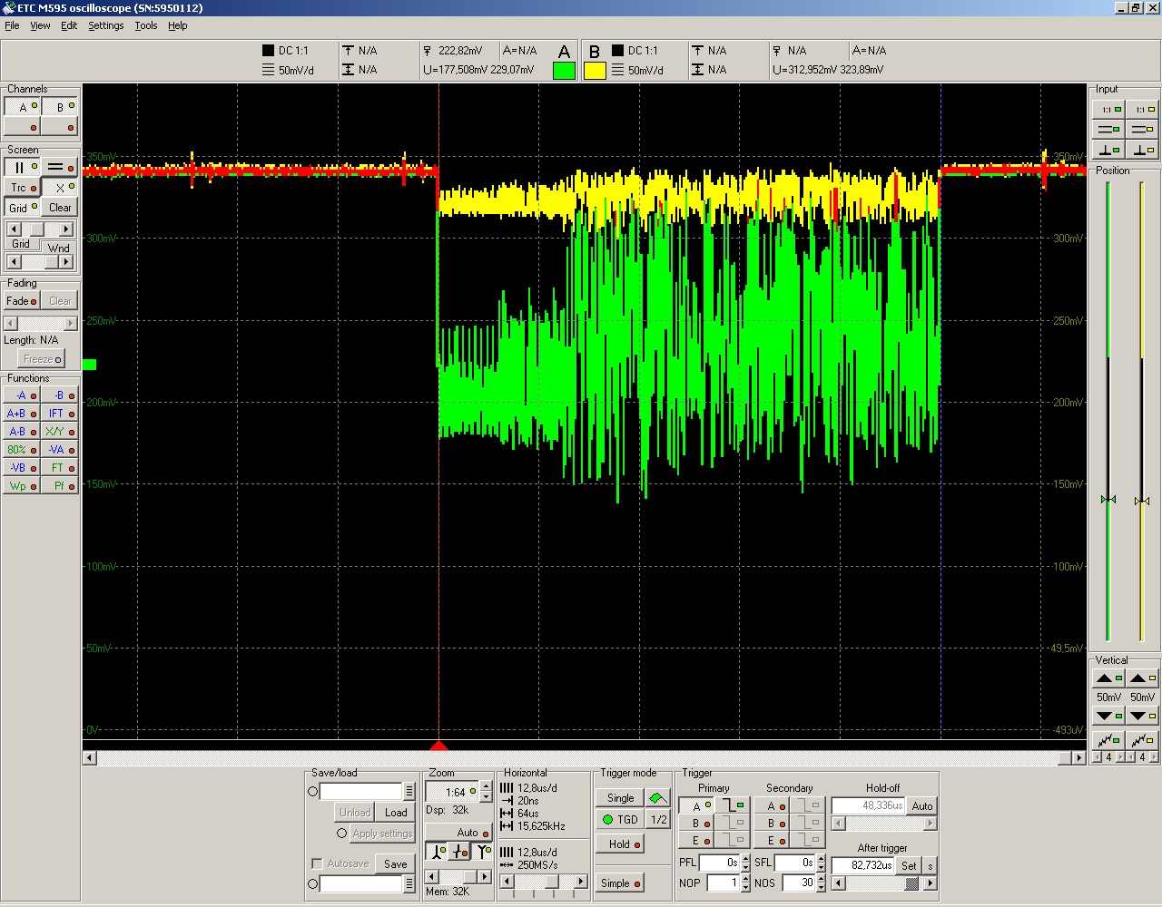
Finally, let's have a look at some 'scope screenshots.
All pictures in this chapter can be clicked to get a full
scope screenshot.
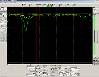
An okay match - coupler terminated
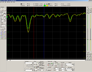
A bad match - coupler open ended
(Maybe I had the probes swapped here - not sure anymore)
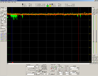
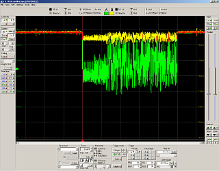
A 1500B ping
The ping sequence is a sample of normal payload traffic.
Note how low the signal level is. Probably a sign of automatic
level adjustments. Apparently, only a select few service frames
(beacons, probe requests?) are transmitted at full TX power.
Also note that you only see the ping request (made by the client
towards the AP) = the TX part. The signal level of the RX response
makes it drown in the noise, as far as my "scope" is concerned anyway.
Note that at 320 us/div, the 1500B frame takes almost a whole
"div" of the scope timebase. The short frames around look like
WiFi ACKs to payload traffic, or perhaps they're something
completely different :-) My typical response time to a 1500B
ping over wifi is about 3 ms, which would match the observation.
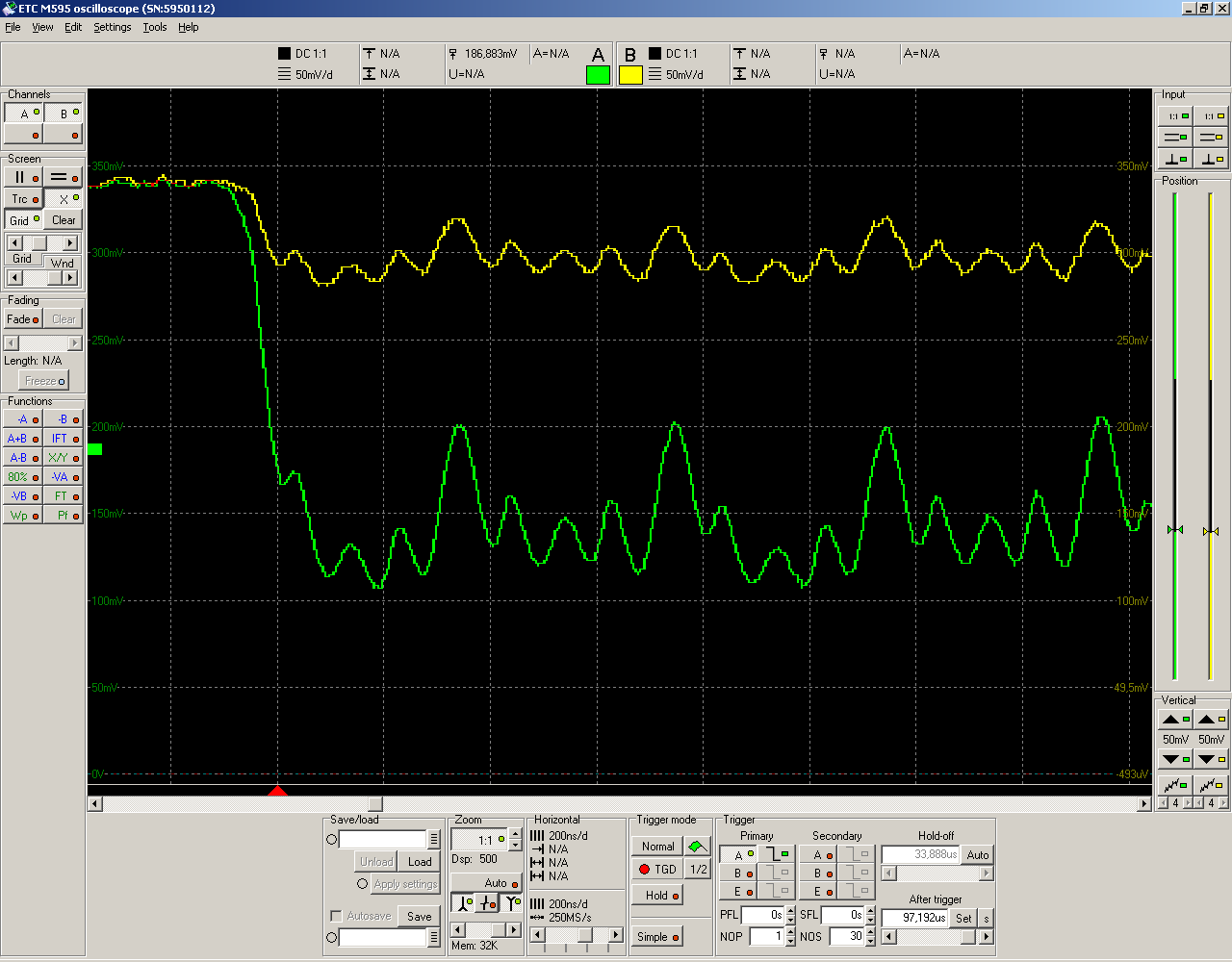
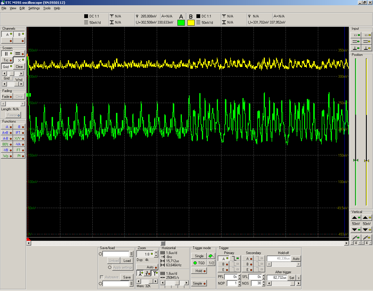
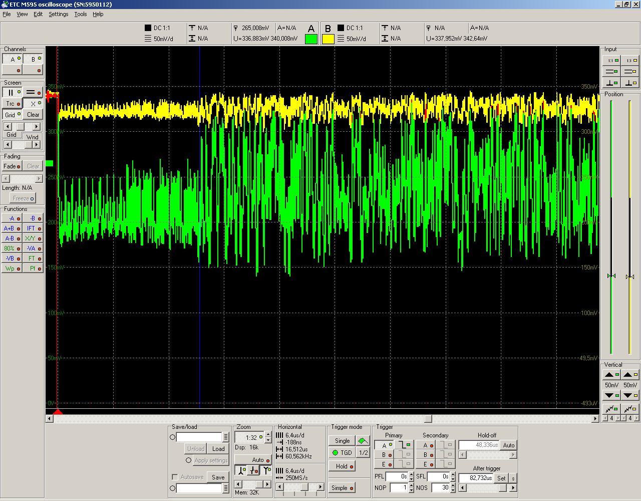
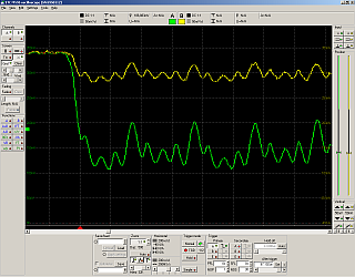
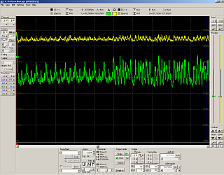
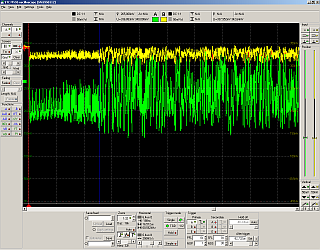
The following scope screenshots probably show some sort of a service frame,
transmitted by the client at its full (nominal, configured) TX power.
Not sure what it is (didn't bother to sniff these) - might be a probe request.
In these frames, the output port of the coupler is attached to an antenna.
Based on the ratio of the two traces, the impedance matching seems okay.
Frame zoomed in all the way
Frame zoomed in some
At this zoom, the screen spans almost the whole preamble
Frame zoomed out some
The preamble (short + long) is framed by the cursors
Frame zoomed out all the way
Mind the prominent preamble at the start of the frame.
In this particular case, it contains two sub-sections,
called "short" and "long", 8 microseconds each,
for a total of 16 microseconds to the combined preamble.
The preamble length of 16 μs is typical for 802.11a;
other 802.11 modulation schemes ("protocol generations")
use different preamble lengths.
The preamble is a "pre-defined scratchpad", for a receiver
to adjust its RX gain or rather to know the signal level
for the rest of the frame. Yes, this "passive RX level training"
happens on a frame-by-frame basis.
Conclusions
As I fiddled with the antennas, terminators, pigtails,
conversion plugs and cables, holder brackets and whatnot,
I have noticed that especially the antenna (SWR indication)
is pretty sensitive to a touch by bare hand, or to metal
objects placed near by, and the extent of the effect depends
on precise geometry of the imperfections in the space surrounding
the antenna.
I have also concluded that the chassis, the antenna holder
and the pigtail length can play a significant role in the
SWR observed by the receiver. If there is a ground loop
comprised of the pigtail shield and the chassis ground,
the loop will form an antenna of its own. You can then
observe effects depending on pigtail length, such as
that an open-ended TML reads as a perfect match,
and a resistive terminator reads as a perfect reflection...
Clearly the pigtail has no problem acting as a "balun"
or an impedance transformer, and the pigtail shield
is by no means some rock solid, objectively given earth.
Gives you some serious grain of salt, if you're in love
with aluminum boxes for your Routerboards :-(
Another observation has to do with pigtail lengths.
The typical pigtails are approx. 25 cm long.
I have noticed that a tight bend on the pigtail
can increase its attenuation.
I have also noticed that I can gain up to 10 dB of
signal strength (realistically more like 8 dB)
if I shorten the pigtail by 10 cm to about 15 cm
= cut to the desired length and rework the RPSMA
female (desolder, clean up, resolder).
But there is a catch: attenuation improves VSWR
as seen by the radio (WiFi transceiver). A mismatched
antenna is less of a problem if attached by a
long long pigtail. By shortening the pigtails,
I could actually harm the TX PA's if the SWR
of my antennas was somewhat bad :-( Combine that
with the aforementioned effect of ground loops
and it's clear that I'd perhaps be better off
if I leave the pigtails rather longer...
Also note that the coupler and any necessary
conversion plugs make the antenna downlink longer
(add to the pigtail length) and disrupt any geometry
that the system may have when hooked up for production
(= without the coupler). I.e., with the coupler attached,
you're not measuring the same system that exists
without the coupler :-(
References
In no particular order, here are some interesting links
revealed by Google while I was doing the "background
research" for my lab adventure and for this paper:
Simple 2.4 GHz SWR Meter published by the GBPPR - my key inspiration
Microwaves101 on VSWR
802.11 OFDM Overview
- apparently a product help chapter by Keysight. Has an interesting and correct description of the WiFi frame preamble.
PCB directional coupler for SWR protection of SSPA up to 1 kW level - has some nice photoes of several coupler PCB's.
SWR Meters and coupler PCB's at WIMO.COM
Playing with S-parameters and the Smith chart in Qucs
By: Frank Rysanek [ rysanek AT fccps DOT cz ] in January 2017