By: Frank Rysanek of FCC prumyslove systemy s.r.o. <rysanek@fccps.cz>
This article started as a braindump after a particularly fruitful debugging session, with some followup reading and further homework - to help me sort my ideas by writing them down, to record them for later reference, and to get them published for the benefit of others. It is by no means complete, the information isn't ready to be set in stone. Rather, it leaves a couple questions itchingly unanswered, and maybe suggests further features to be implemented in some proprietary RAID firmwares and in the open-source Linux (IO schedulers). Any feedback on this text is welcome, maybe especially negative.
The aforementioned "research" (cough) was prompted by a particular customer case, which presented us with some tough questions regarding a RAID unit that we were trying to sell. The RAID unit had to face a particular difficult type of load from its host server. Such is the basic context of the arguments presented below. My focus will be on server loads requiring high sustained throughput, potentially for many parallel client sessions - the conclusions in the scheduler tuning paragraphs are likely irrelevant if what you're after is a snappy desktop experience :-)
Any data given in this article are valid roughly "as of the time of this writing". If this paper remains exposed on the web for several years (as has happend to a number of my previous pieces), some of the data will likely get gradually skewed against future reality - so take them with a grain of salt. Today is March 20th, 2009. And of course, you can never exclude a "quantum leap" to a completely new technology (not sure Flash SSD's are the right example).
When testing (performance of) disk drives and RAID units, I'm using an in-house block device level tool called hddtest (for Linux). A few months ago, it has reached somewhat publishable quality. Source code (GNU C++) is available here:
hddtest-1.1.tgz
Warning: using the -w switch, hddtest will erase your hard disk!
Hddtest merely reads or writes the drive and shows some simple instant throughput figures (user space level). Combine it with smartctl, iostat and maybe hdparm to get a thorough view of your hard drive's health, block-level runtime traffic and configuration features.
I've also pieced together a quick snippet of C/C++ code that simulates the "parallel sequential streaming load". It first fills the filesystem with large files, then it launches some threads to slowly read and write individual files sequentially (each thread picks one file at random). Here it goes:
http://www.fccps.cz/download/adv/frr/paraseq-0.1.tgz
Warning: paraseq without parameters will try to clog your filesystem with huge files, and then eat all your free RAM and CPU!
Bug reports are welcome, especially those coming with a patch :-)
The basic mechanical construction of a classic hard drive is notoriously known, there's little point in reiterating it here. There's a revolving spindle driven by a motor, and one to four platters, single- or double-sided (accessed by one or two heads per platter). The heads are positioned over the platter surface by an arm (or a stack of arms) on a hinge, deflected by a strong electromagnet. There's a single PCB with drive electronics, slapped onto the underside of the drive, i.e. outside of the "platter cleanroom".
The heads don't read in parallel - only one head of the total headcount is active at any one time. So the outer sequential rate of ~100 MBps comes from a single head. The track seek alignment operation is likely too sensitive to allow for simultaneous precise positioning of multiple heads over their respective multiple platters - all the head deflection arms are mechanically stacked and bolted tightly together and moved about by a single common electromagnet.
Today's hard drives essentially keep constant platter RPM during operation (except for some recent power-saving adventures). At the same time, to keep spatial linear bit density constant under the head, the inner tracks have a lower capacity per track, and give a lower runtime bitrate (bps). All drives give a higher sequential transfer rate at the start of the LBA disk space, and if you care to read the whole surface, by the end the rate drops to maybe as low as 40-30% of the initial sustained rate. The onboard cache is far too small to cause this effect. The obvious conclusion is, that the drives read the platter space from outside inwards (i.e. in an opposite direction to e.g. a CD).
This may have psychological / marketing reasons. To the casual tester, or just after deployment (empty filesystem), the drive will appear faster. But, it's also a notorious cause of later disappointment - as the filesystem gets gradually full, this is yet another factor contributing to the typically percieved slow-down.
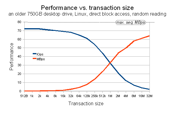
The following chart shows some practical results of a somewhat recent disk drive.
Interestingly, as the technology develops, the sequential MBps continue to grow with sqrt(capacity), but the IOps do not! Sometimes a recent-most drive with bleeding edge capacity can have lower random IOps than a drive that's a generation older. Also, note what the capacity growth does with "IOps per TB", which is a valid indicator to some users.
As mentioned before, in the long term, sequential MBps grow roughly with square root of per-drive capacity - or more precisely, square root of per-platter bit density (bits per square inch). My first 100MB IDE disk drive by ALPS used to achieve about 600 kBps. My later 1.2GB Quantum Fireball gave about 2.5 MBps. The current 1TB drives are around 80 to 120 MBps. Obviously within a single drive family and generation, among drives with 1/2/3/4 platters (capacities quite varied), the per-drive sustained transfer rate is equal, as only one head at a time is active, and the platters have an equal bit density. As a side note, drives with lower platter count consume less power and tend to have slightly faster seeks. The square root alone has interesting consequences. It took maybe 4 minutes to read the whole of my first 100Meg Alps drive. My second Quantum Fireball took maybe 10 minutes to read. The 1TB drives of today take over 3 hours to read! And, that's sequential throughput. If you consider random IO, you feel like you're sipping a swimming pool with a straw.
Note that the IOps figures in the above graph are inversely proportional to a somewhat credible average per-transaction completion value, easily substitutable for average seek time. Hddtest feeds the output of /dev/urandom into the seek position sequencing algoritm. Thus, the resulting averages are not based on some "typical application usage patterns", but are based on (almost) perfectly random seek positions. The seek times thus produced (or, rather, transaction completion times) consist of several components:
ttot = tcomm + tseek + trotational + ttransfer + tos
When reading from system cache, the OS can achieve hundreds of thousands of IOps to a single user-space thread. When reading sequentially from a drive, a single drive can achieve thousands of IOps. As a consequence, the communication time and OS handling delay are comparably negligible under random IO scenarios, where the drives typically max out at low hundreds of IOps. For small transaction sizes, the transfer time can also be neglected. So we're left with a sum of the linear seek time and the rotational latency (half a revolution on average), which is clearly a good indicator of the drive's bare seek capability.
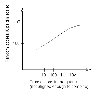
It probably makes you wonder if it would be possible to make life easier for the drive, by making the seeks somehow shorter, by making the consecutive IO transactions packed closer together in the disk space. Yes, that's definitely possible, read more on that below, in the chapters on caching and IO scheduling. If you provide a deep IO queue in the host OS, combined with request re-ordering, the seeks do indeed get physically much shorter. The results can be surprising - or rather, surprisingly small. E.g., the aforementioned nameless 750GB drive never exceeds about 200 IOps, regardless of how deep your OS-level IO queue becomes. Tested with queue depths on the order of 10000 or above, with WB cache volumes over a GB... the average seek time just didn't scale. See the following chart.
This likely makes you wonder even more. How come? Is the drive internally so CPU-starved? Hmm. Maybe not exactly. Consider rotational latency. 7200 RPM, that's just over 100 revolutions per second. An average rotational latency is half a revolution, i.e. it should allow for over 200 IOps. Which is already close to the observed result. Apparently NCQ doesn't help much for some reason (NCQ was ON in this test).
Note: an important condition to get this result is, that the load generator produces seek positions that are random enough - i.e., that write-combining doesn't reach significant level. Write-combining avoids rotational latency.
In terms of random access, drives typically show a slightly higher write throughput than read throughput - possibly owing to the fact that writing allows the drive to use write-back caching combined with queued dispatch. In terms of sequential access, the results are similar between R/W, slightly varied among different disk drive models.
Disk drives are not born equal. There are "desktop" drives and there are "enterprise" drives (read: drives for servers). In general, in a comparable form factor (say 3.5 inch), desktop drives have higher capacity and lower throughput - lower especially in random IOps. For example, a 74GB 15k RPM drive could give 130 MBps peak sequential throughput and 150 IOps random read throughput (170 IOps random write). So the difference is significant, though maybe not dramatic. And, enterprise drives are more expensive per unit.
If you take a look at the under-the-hood thumbnail photoes at www.seagate.com (on top of every product page), you may notice that desktop drives have larger platters, maximizing platter square. Enterprise drives have a smaller outer platter diameter and a larger inner diameter of the active platter area. This corresponds with the fact that enterprise drives show less "sequential MBps degradation" between disk space beginning and end - the end is at maybe 60-70% of the initial MBps, compared to 30-40% of a typical desktop drive. Enterprise drives are supposedly also made of better quality materials and are otherwise optimized for both higher IOps and longer endurance. Note the difference in typical platter RPM for instance - a few years ago, desktop drives revolved at 5400 RPM, nowadays 7200 RPM is the standard. Enterprise drives are at 10k or rather 15k RPM. The platter size alone is perhaps not enough to explain the great difference in maximum drive capacity between desktop and enterprise drives. Data density (bits per square inch) and the corresponding track density (tracks per inch) are another likely factor to both seek performance (at lower track density, track seek settling time can be lower) and durability (less dense tracks are less sensitive to vibration). Lower head count (platter count) can also mean faster seeks - fewer arms, deflected by the same electromagnet. Enterprise drives may have a stronger electromagnet, again for faster seeks - facilitated by less stringent accoustic limits in server environments.
An important point in server deployment is, that sometimes the total capacity is less important than random IOps capability. Or in other words, a huge total capacity is no use, if you cannot read it at the transfer rate required. If your storage subsystem doesn't have the IOps required, your magnificent total capacity is effectively unreachable. In such cases, price per TB is clearly not the key criterion. More on that below, in the chapters on RAID configurations and IO scheduler tuning.
Besides the classic desktop and enterprise categories, there are various crossovers.
Traditionally, enterprise drives had a SCSI interface (later superseded by SAS) and desktop drives were limited to ATA (later superseded by SATA). Command queueing was first introduced in enterprise drives (TCQ with U160 SCSI), later got adopted into SATA in a somewhat stripped-down form called NCQ. Nowadays you can meet drives that are desktop grade by mechanical ancestry, but come equipped with a SAS interface.
There are also desktop SATA drives with a slightly different firmware (and possibly more stringent QC and longer warranty), sold as entry-level RAID drives. Though their sibling desktop drives work equally well for many purposes.
And finally, there are "enterprise SATA" drives, that supposedly have an enterprise-grade mechanical construction (witnessed by the typical "enterprise" capacity raster), coupled to a SATA interface. Combined with 10k RPM. Yes I'm talking about the Raptor drives. Take the Velociraptor for example - another weird feature of the drive is, that it's actually a 2.5" drive in a 3.5" heatsink. The initial version didn't even fit in a 3.5" SATA hot-swap drawer, the current version does (it contains an additional conversion connector to achieve that). By that description and also based on price, you'd expect IOps numbers somewhere between a desktop drive and the classic enterprise models. Yet it seems that the drive can do better. A basic random read test with 64k transactions gives about 130-140 IOps - not exactly an extreme figure. A basic write test shows about 240 IOps witht 64k or about 270 IOps with 4k sectors - that's already a bit of a shocker. But if you can provide a deep enough IO queue in the host OS, making the physical seek discance real short, that's where you can get a mighty shock - the drive can deliver up to 580 IOps in 4k random writes... that would seem to defy basic HDD physics! I mean, rotational latency. As if the intra-revolution NCQ seeks spanned a particularly wide area of neighbor tracks.
Somewhat ignorant of the ongoing desktop vs. enterprise rage, there's yet another category of disk drives: the notebook disks, with their classic 2.5" form factor. Traditionally, these are disregarded as slow, only any good for mobile and low-power applications. Nonetheless, technically speaking, a 500GB drive that gives 70 MBps sequential and 55 random IOps is not all that slow by me :-)
In modern computer systems, disk IO caching takes place at several levels: in the host OS (using the computer's physical RAM), at the RAID level and within the disk drive.
At the OS level, in modern-day operating systems, IO caching is an inherent/integral part of the disk IO software paths and virual memory mnagement. The IO cache can occupy all available system RAM that is currently free from user-space apps and kernel-space allocations for a particular purpose. If the system needs more RAM for the applications or some kernel-space purpose, it's very easy and "cheap" in terms of CPU time to clear some pages currently in use for IO read caching (i.e., pages that are not "dirty").
True hardware RAID controllers are typically based on a small embedded computer. A RAID card in a PCI slot is essentially a small autonomous computer within the bigger host computer. As such, the RAID controller has some RAM that is used for firmware code execution and especially as a RAID cache. In the more expensive RAID controllers, the volume of the RAID RAM can be upgraded - the RAM is in the form of DIMM's or SODIMM's. Obviously this RAID RAM is dedicated to the IO caching function. Note that striped RAID levels with parity (such as RAID 5 or 6) need caching at the "host side" (the host's IO transactions) and at the "drive side" (stripes and stripe sets) of the RAID engine - striking good balance between the two RAID cache compartments, or some dynamic on-demand cache allocation for either side, is likely key to swift RAID operations, and indeed various lower-end RAID implementations do differ in their cache throughput even on the same hardware (same IOP CPU, same HBA chips, same volume of RAM). Host-side caching is key to maximum host-to-cache access (both reads and writes), and drive-side caching is key to maximum write throughput with sub-stripeset-size writes and read-ahead.
Every disk drive has some volume of RAM as well. In the near history, this has developed from some hundreds of kilobytes through typical values of 2 or 8 MB to the today's typical capacities of 16 or 32 MB. These onboard RAM buffers are dedicated to disk IO caching.
The effects of basic read caching are clear. The IO cache holds data that has recently been read from or written to a disk, and if some application needs that data again, it is instantly available from the cache. Modern-day operating systems would be very slow without inherent OS-level IO read caching. Given the typical relative sizes of RAM (cache) in the host computer, a RAID controller and the drive itself, read caching is perhaps most important at the OS level - except maybe for computers running fat and greedy applications that eat all available RAM (in such scenarios, a beefy RAID controller with lots of dedicated cache is a good way to provide some cache out of reach of the host computer's greedy user space). In RAID controllers, effective read caching also helps to improve write throughput in striped RAID levels with parity (e.g. RAID 5 a and 6) on small write operations, if the neighbor stripes for a stripe set are in cache, they needn't be read from disk ahead of the necessary parity calculation and write-back.
Read-ahead is a speculative algorithm, where the particular I/O layer reads more data than actually requested, in the hope that the application will read more data from the same file (or block device) in the near future. If that happens, the data is instantly available, owing to the read-ahead algoritm.
The potential downsides of read-ahead are additional consumption of RAM (read cache space) and increased transfer time in the total seek time formula.
Nevertheless, e.g. in modern disk drives, it doesn't make sense to disable the read-ahead feature. Without read-ahead, the drives are slower in terms of sustained sequential MBps (by maybe 20 per cent), and with tiny transaction sizes the low-level random IOps capability is the same with or without read-ahead enabled. Maybe this shows some intelligent / adaptive behavior in the drives' read-ahead algorithm. Read-ahead on sequential loads (series of back-to-back requests) allows the drive to keep reading, without waiting for the host computer to send the next read request (and then waiting for the platter to revolve back to the right angular position).
In RAID controllers, the read-ahead algorithms also tend to be more or less adaptive, and sometimes read-ahead can be explicitly turned off. Recent Areca firmwares offer three levels of read-ahead (plus "disabled").
At the OS level, in some OS'es the read-ahead function can be tweaked (certainly in Linux).
Overall if you're struggling with highly random load, it can be useful to fine-tune the read-ahead function at least at the OS and RAID level.
Also called write-behind caching. An IO write syscall immediately returns to the application with a success result code, but the write transaction is actually postponed, stored in cache to be processed later, when suitable.
This approach allows for sky-high write performance - that is, unless/until the volume of write-back cache memory runs out. Especially under highly random write-heavy load, the drives may not have enough IOps to keep up with the application generating the load. When the WB cache volume runs out, the write() syscalls start to get blocked until some transactions are dispatched to the disk drive.
The write-back mechanism effectively turns all the writes (submitted in a blocking way by the application) into asynchronous/non-blocking transactions - as such, they can be effectively queued and re-oredered in the queue for optimum sequencing/scheduling to the disk drive.
Also, within a disk drive, write-back caching is key to reasonable sustained transfer rate. WB caching allows the drive to queue several transactions internally, even without TCQ/NCQ in the outer interface protocol, i.e. ATA drives can do it too. This ability to gopher several upcoming transactions allows the drive to have the next chunk of data instantly available in long sequences of consecutive writes - thus the drive can write data to the track without any hesitation, i.e. without inserting additional rotational latency between transactions. If there was no write-back capability, the drive would write a chunk of data, confirm transaction to the host computer, wait for it to send another chunk of data, then wait until the platter is done revolving back to the required position. In the ancient days of MFM/RLL and early ATA drives, this was addressed by an explicit "sector interleave" mechanism.
IO command queueing in itself is perhaps not a cache algorithm, but it is closely linked to write-back caching. Command queueing and re-ordering again happens at all the three levels (OS, RAID, disks) and the queued IO transactions can be of various types: writes, reads, and even various device management transactions. The reordering part of queueing is handled by a piece of software called the "IO scheduler".
Write-back traffic is particularly easy to queue, as mentioned before. Even a single writing thread can make full use of the queue depth available. Read requests are typically a different matter. A single program thread typically asks for reads in a blocking (synchronous) fashion - another read request is not submitted until the previous request has returned. This leads to explicit serialization of the transactions, there's always just one read request per thread in the system IO queue - thus, there's no way to re-order read requests for a single thread in the system queue or at RAID and disk level. That is, unless you consider "async IO", which is a fairly novel concept and API, at least in Linux. An important way around this limitation of read requests is to use multiple reading threads in parallel, if the natural flow of data in the application allows for that (like various server applications for LAN or WAN use). In a system-wide per-device IO queue, the individual blocking read requests coming from multiple threads can be reordered and dispatched irrespective of their original submission order.
In a RAID controller, the queueing function is fairly boring and obvious (and if not, the algoritm is proprietary / closed-source anyway).
In a disk drive, at a first glance, queueing and the associated re-ordering has the same conceptual possibilities and goals as at the OS and RAID levels. That is, order the writes by LBA address, thus to minimize the physical seek distance and hence also the average seek time. At least the classic IT textbooks describe the disk drive operations strictly in terms of "track seek, then rotational latency". Yet it seems that TCQ/NCQ may mean something yet more refined: modern drives are supposedly able to seek multiple times within a single revolution (obviously just among a very narrow set of neighbouring tracks), thus minimizing the rotational latency.
Therefore, arguably it makes perfect sense to have a cascade of multiple queues at the aforementioned levels: OS, RAID and disk drive. The OS and RAID levels prepare a tightly packed and ordered sequence of transactions, and the drive still has opportunity for local intra-RPM optimizations over a small range of consecutive IO requests.
Write combining too is more of an IO scheduler algorithm than a cache concept. Consecutive back-to-back IO requests of the same type can be merged into a single bigger request, before being submitted to the lower IO layers. This is performed at various levels: already in some parts of the user-space libc (file IO vs. low-level file descriptors), certainly in the OS-level scheduler, likely also in the RAID and probably/effectively also in the disk drive itself. Actual write combining saves some processing horsepower and communication time at the lower layers, thus potentially allowing the overall system to achieve greater user-level IOps - especially if the application is poorly written, generating lots of small but consecutive transactions at the source code level. In "queue full" scenarios, the fact that requests are combined can save some "queue slots", thus again achieving higher IO throughput.
Please note however, that even some basic ordering and back-to-back packing of requests (while keeping them separate entries in the queue) provides significant perfomance improvement, as the disk drives appreciate an ordered stream of consecutive adjacent requests much more than sparse or even random data, and pay off with much higher IOps values. So with the exception of "queue full" conditions, further write-combining typically yields little benefit.
The overall basic notion is that caching is always a good thing, and that more cache means more throughput. If your flock of spindles become a bottleneck, just throw some more cache RAM at it and the problem will go away. Any throughput problem can be solved with more cache.
Well, not necessarily, it depends. Some load patterns can prove particularly troublesome. Often it turns out that no reasonable cache volume alone can help you, unless you consider cache sizes comparable to the total disk space (and even that may actually prove insufficient). Instead of thinking "big storage boxes with huge cache", try to sit back with a mug of coffee, analyze your load patterns and try to massage/architect your set of spindles to match your load pattern, possibly using some cache+scheduler+RAID based transformation. It only takes basic knowledge of disk drives and some rather basic math.
A side note on cache memory: today's lower-end RAID units and PCI RAID controllers typically take DIMM (or SODIMM) memories - with ECC, but otherwise easily available and relatively cheap (maybe several per cent of the total RAID unit cost). Note that for any memory technology (SDRAM/DDR/DDR2), there is a certain "maximum economical and normally available DIMM size", such as 1 GB for DDR or 2 GB for DDR2. Higher capacities may be in the price lists, but the price per MB is twice higher and availability is questionable. And, generally it's much easier and cheaper to stuff more RAM into the host server, than into a reasonably expensive RAID controller.
... as seen e.g. in file servers. This is perhaps the easiest type of load to be satisfied by a generous cache size. If the cache is big enough to take some bursts and store them later, it doesn't get any better. Basic read caching helps serving particularly popular files. Choice of disk drives is up to the system admin - depends on the size of the network or audience served, on preference of capacity vs. IOps etc.
This is still a fairly easy load to handle. A single source of sequential data, often providing as much data as the disk subsystem can take. This is typical for video grabbing and simple processing applications. Huge cache is really not much use, as it will get choked anyway - the sustained MBps throughput will settle on the narrowest bottleneck, which is often the RAID controller's XOR accelerator or bus throughput, hardly ever the disk drives (unless you're using bare drives). Yet a good cache volume does have some merit, as a video stream funneled through a filesystem layer produces some random out-of-sequence metadata writes (often ordered by IO barriers - oh well). The amount of stream randomization added by a filesystem depends on the filesystem type (does anyone have a comparison of HFS+ against XFS? :)
Use a RAID unit model that satisfies your basic sustained sequential MBps requirement and load it with as much RAM as economically reasonable - which nowadays can mean the maximum volume available on the market with a short delivery lead time :-) As for disk drives, today's SATA drives are usually plenty fast enough for this application, as long as some data safety measures are taken (RAID with parity and possibly some backup framework, if operationally viable). Use enough drives to satisfy your total sequential MBps requirement (sum of individual disk drives, with some added slack). With cheap desktop drives, make sure their sum is fast enough even at the slow grim end (innermost tracks).
Sequential reading in a single thread again needs relatively little cache. Sequential read-ahead only takes a few hundred kB, the rest will get trashed over and over. Yet if you're doing some editing / processing on the data, voluminous RAM in the host system and in the RAID may prove useful.
Most database loads are highly random. RDBMS engines often prefer to handle their own IO in direct mode, avoiding the OS-level buffering and IO scheduling. This is both for safety and performance reasons. There's little to be gained from a big system-wide cache for completely random reads from a much bigger pool of disk drives (the cache gets trashed). Often the RDBMS can cope with the drives directly, rather than through a RAID of some sort. If RAID is to be considered, the most popular choice is RAID level 10, with stripe size set to match the VM page size of the host machine or of the RDBMS engine. RAID levels with striped calculated parity (5/6/50/60) should only be considered for very performance-relaxed and cost-sensitive deployments - random write operation of those RAID levels is abysmal, more on that below. Same point about choice of disk drives. Random IO unfortunately hinges on IOps capability in the first place, capacity possibly second. "Unfortunately", because maximum IOps capability is available from the "enterprise" variety of drives, which are more expensive per spindle than desktop drives.
If you need more random IOps, consider adding more spindles. With direct RDBMS use or with RAID 0/10, the IOps figure scales fairly well with the number of spindles, as the transactions get somewhat randomly distributed among the spindles. This is true about both reads and writes. That is, provided that the RDBMS engine generates the read requests in an async/overlapping fashion, which is almost always true. With the aforementioned calculated-parity-based RAID levels, read performance scales fairly well too (with the spindle count) - as long as the RAID volume is healthy. Think about this if your database is "read-mostly".
Some databases, relational or otherwise, are used to store bigger chunks of data. In that case, feel free to vary the layout of your storage back end - RAID level, stripe size etc. If your database shall store both relational and blobby data and you're concerned about performance, consider setting up separate RAID volumes for the relational (highly random) data and for the blobs (semi-sequential), possibly with different RAID levels and chunk sizes. And map the tables to those table spaces accordingly. Your RDBMS will thank you.
This is a tough one. Imagine a busy FTP server for instance, with both uploads and downloads going on in parallel. Although the natural organization of the data on disk is sequential, the interspersed arrival of the streams makes the load look highly random in the short term. The data can flow in and out as fast as the network interface allows - a single GbEth port theoretically yields up to 100 MBps full duplex, but you can have multiple GbEth ports in a single machine, or a 10Gb port. Current low-end RAID controllers from various vendors, based on the Intel IOP341 / 348 family (or some alternative competitive architectures with comparable throughput) with the cheap SATA drives can provide say between 600 MBps and 1 GBps of sustained sequential throughput all the way to the disk drives - just about enough to choke a 10Gb Ethernet, provided that the load is shoveled to the drives in a highly sequential manner.
So you have 100MBps+ worth of traffic, flooding your server from the whole wild internet. In the short term, the data corresponds to very random seek positions - with a prospect of pulling some longer-term optimizations, if you can track the individual sessions and optimize them into bigger IO transactions against the individual disk spindles.
Cache volume alone doesn't help - generous cache is certainly a basic requirement, but you need to fine-tune the chunk sizes, RAID level (or your overall disk pool arrangement) and the precise behavior of the various caching methods employed at the multiple levels of your disk IO subsystem. Some basic application-level sanity is also highly advisable, in order to save RAM, CPU horsepower and IOps.
In order to get close to sequential performance in terms of MBps, you need to massage your load into some minimum chunk size. Based on the chart above (in the chapter on disk drives), such a reasonable chunk size might be 4 MB or maybe more. Only such a big chunk size eliminates the random IOps bottleneck. Such big chunks, if accessed in a random fashion, yield a "close to sequential" MBps throughput.
Next, make your OS or your RAID read data in chunks of this size - so e.g. those 4 Megs are your desired read-ahead size. Multiply that by your maximum number of simultaneous reading threads and you get the necessary volume of RAM for additional read cache. Somewhat surprisingly, the desired read-ahead behavior can be pretty difficult to achieve in practice. For the moment, suffice to say that you need intelligent per-file read-ahead, which doesn't map very well to the crude and clumsy block device chunks and block-device-level read-ahead...
For writes, somehow you need to persuade your server app or OS or RAID to write-combine the tiny trickling per-thread packets over a long period of time. This can be done by equipping the system by a massive volume of cache and by trying to fine-tune the OS-level or RAID scheduler for maximum scheduler queue depth and maximum write-back "patience". Note that the relatively small outer TCQ depth of a SCSI-attached HW RAID controller is not much of a problem, as long as write-back caching is enabled on the RAID controller. Again, take your desired average burst size and multiply by the number of simultaneous write threads, to get the desired volume of dirty cache being slowly flushed by the write-back scheduler. It sounds complicated, but it turns out to be relatively feasible in practice.
Obviously it helps if the filesystem used makes maximum effort to make the data allocations continuous/contiguous on the drive, at least on par with the RAID chunk size (4 Megs or above in this case). Some FS types are better at this than others, e.g. XFS is reputed for highly contiguous allocation. The writing application threads should also make it easier for the FS to keep the data unfragmented, e.g. by using syscalls such as fallocate()/fadvise()/madvise() at appropriate points in the code. Note that fallocate(), which may sound like "just the right thing to do if you know the file size in advance", actually causes the kernel to dump a sequence of zeroes to the file (and block until that is finished), so it delays the start of your app's actual writing and really doubles the data volume written to the block device. For most practical purposes, this behavior is not what you want :-( Also, fadvise()/madvise() seem to have a relatively limited effect, nowhere near the 4MB chunkiness/contiguity that we're after.
RAID levels with calculated parity (5/6/50/60) are again impractical. A write in those RAID levels is only somewhat effective if a whole stripe set is written at once (or multiple stripe sets in sequence) - so that the RAID engine doesn't have to read ahead the unchanged stripes from all the spindles. In other words, a write into these RAID levels makes all the heads seek in sync (possibly for two consecutive transactions), thus reducing the available total IOps available from the affected spindles to a fraction of the usual sum. Making the stripe sets short does help a bit (half the number of disks in a set means twice the IOps), but that's not very much and certainly at the expense of data safety. Besides, speaking of huge RAID stripe sizes (to avoid the IOps bottleneck), note how huge the stripe sets would become - and the write is only somewhat effective if a whole stripe set is written en bloc. Note that aligning the writes to stripe or stripe set boundary is effectively impossible (compared to read-ahead, which tends to be well aligned), which hampers efficiency even for over-stripeset-size writes.
Therefore, if the disk subsystem is to be load-balanced using a RAID, it should probably be level 10, where writes are almost equal to reads in terms of IOps cost (well, twice as expensive) - unless your system is highly "read-mostly" and a calculated parity RAID can be coped with.
Most hardware RAID controllers have a maximum stripe size somewhere around 128 to 512 kB. I.e., nowhere near those 4 MB minimum. Perhaps the most easily available RAID that's capable of chunk sizes around 4 MB is the classic Linux MD RAID (configured using mdadm). Yet it may be advisable to use a hardware RAID unit even for the basic mirrors, to provide comfortable hot-swap and rebuild for faulty drives (and combine the HW mirrors with a Linux-based SW RAID 0) - that is, until Linux gets flawless drive hot-swap handling up to the software RAID, with or without SCSI Enclosure Services support (which has already appeared in Linux 2.6 kernels). Drives do fail - the question is not if, but when and how often.
If this is e.g. a web application with some programmatic control over data placement, the system designer/administrator should also consider yet another arrangement: using several stand-alone mirrors mounted separately to different mount points, with application-level distribution of files to the individual mirror devices. This cancels the fixed chunk size necessary for any striped RAID level (including level 10), and allows for the arbitrary-length ordered write-back bursts from the OS-level IO scheduler to always flow sequentially to a single disk drive. Note that this arrangement does not cancel the requirement for contiguous file space allocation - the apps should take some measures to keep FS fragmentation low, if at all possible. Also note that this arrangement is potentially sensitive to local bottlenecks - if a particular file becomes extremely popular (and is too big to stay in the system cache), a single drive may become a bottleneck in the system. Imagine a new release of a Linux distro being rolled out to the master servers. Yet it won't block access to the other spindles, so other downloads may crank away all the happier... Still, where such inhomogenities are a problem, perhaps RAID 10 with a huge chunk size is more appropriate for a more even load distribution among the spindles.
Note that the Linux DeviceMapper+LVM2 is not a very practical choice for the purpose of merging the mirrors into a PV pool - the chunks are 4 MB large by default, but they're kind of "virtual", allocated in a consecutive fashion (as a single long linear range per PV), so that unless the filesystem is always full, the IOps and MBps load would not be distributed evenly among PV's (spindles). The DM-mirror module is also not quite an option, as it's limited to 512 kB of stripe size. Using bare DM-linear to set up individual 4MB chunks on different drives is not a good idea either, as the number of linear 4MB LBA ranges would be too high to be practical...
Another thing to note is that if your block device is a striped RAID with huge chunk size (say 4 MB), you should take care not to create a BIOS partition table on top of that block device, because that way the first partition will typically get misaligned to RAID stripe boundaries. The partition will start at an odd sector number (63), and as the readahead chunk in Linux tends to be aligned to a power of 2 (128 kB by default), the transactions will tend to overlap stripe boundaries. Which will likely degrade the IOps available from your spindles... The simple advice is to use the bare block device to create a filesystem. If only read-ahead size of 4 MB made practical sense in Linux... (more on that in the "tuning" chapter).
Hddtest can be asked to produce sequential or random access load with adjustable transaction size (default is 128 sectors = 64 kB), reads or writes, with or without block device buffering on part of the Linux OS (the latter mode is invoked using O_DIRECT flag to the open() syscall).
The reads are essentially blocking (single threads), unless you run multiple threads on the same block device, which is possible - still the resulting queue depth is not big enough to allow for some massive scaling of random IOps based on physical seek contraction. It's good enough for testing how effective the parallel read dispatch works over striped RAID volumes.
The writes are blocking in the calling thread, but the OS-level write-back and IO scheduling can make them arrive to the block device as if submitted in an async fashion. HDDtest writes at the maximum rate possible - the only blocking call in the loop is the write() :-) Thus, regardless of whether it runs in sequential or random mode, it clutters the system dirty IO cache and writeback (scheduler)with as many IO requests as it is allowed, before the read() call starts to get blocked. Note that this "maximum hog" behavior is not typical for sub-critically loaded servers, and the load it generates is highly random, so it is not a completely valid synthetic load generator for "multiple parallel streamers" scenario. Yet the behavior is good enough for testing the scheduler efficiency in "seek contraction" tests and for hard drive tests with this type of load.
Let me start this chapter with a word of warning.
There are many RAID implementations from many different vendors. Some are cheap, some expensive. Fortunately the RAID controllers are nowadays (finally) strong enough not to be a bottleneck in the system in terms of sequential MBps. Obviously there are still some CPU-starved models on the market and some brands historically had a sub-prime firmware efficiency, but esentially it's no problem anymore to buy a PCI RAID card with a decent enough throughput compared to the disk drives.
The catch can be elsewhere: the basic RAID geometry and simple maths apply to everyone, irrespective of brand and price - just like basic physics. An expensive brand on the face plate or a hyper-strong CPU won't make the spindles seek faster, and a huge cache may only have a limited effect on some loads. Beware of marketing hype, and take care to apply the most sadistic load generator to any hardware that you're allowed to test-drive. Try before buy.
Some high-end storage vendors claim to use special disk space allocation arrangements and parity maintenance techniques that are supposedly superior to the classic humble RAID levels, standardized many years ago. Again, take those claims with a grain of salt. You only have so many spindles and so much cache.
I'm leaving the RAID basics up to other materials (various RAID primers and vendors' usage guides). Let's focus on the gotchas - the maths around IOps and MBps aggregation.
Let's start with the simple case, as it already has some features that also apply to the striped RAID levels with parity.
A practical example: suppose you have 16 cheap desktop disks, capable of 70 random IOps each. The total random IOps capability of those drives in RAID 0 will be 70 * 16 = roughly 1100 IOps. If the stripe size and transaction size is 64 kB, that results in 70 MBps of total throughput (note: this is on par with the sequential throughput of a single drive). It can get somewhat better with heavy request queueing. Write-combining is a double-edged sword, if it makes your request size just climb over stripe size... Enterprise drives give about twice the random IOps, and their IOps number scales somewhat better with deeper queueing (better than with the desktop drives).
RAID 0 stripes the virtual volume space into equal-sized shreds and stacks those shreds onto the physical drives in a round-robin fashion. The single shred is called a "stripe", and N shreds in a row across the disk drives are called a "stripe set".
If you read sequentially from a RAID 0 volume, the RAID controller keeps reading the stripes in a round-robin fashion. As each drive reads ahead a bit and so may the controller, the sequential throughput of the drives gets combined (summed), as long as the busses, memories and RAID controller CPU do not become a bottleneck. Same behavior for writes, under the same conditions.
If you read a random chunk of data from RAID 0, a single drive has to seek, and gives you the data. The seek time achieved is the drive's average seek. Implied conditions: the read transaction size is less than or equal to stripe size, and aligned within a single stripe. Same behavior for writes, under the same conditions.
If you flood your RAID 0 volume with randomly seeking sub-stripe transactions (again reads or writes), the seek positions within the RAID 0 volume are mapped to individual spindles (=drives) at random, and hence the per-drive random IOps neatly sum up (almost perfectly) into the total per-volume IOps figure. Implied conditions: the transactions are again stripe-aligned.
If you flood your RAID 0 volume with random transactions (see above) that are not strictly stripe-aligned, then any volume-level transaction that overlaps across a stripe boundary causes two spindles to seek = consumes two IO's from the total IOps sum of the RAID volume. Hence, if all your transactions are sub-stripe and unaligned, your total IOps figure shrinks to a half. (Which can easily happen with an improper OS setup. More on that in the "tuning" chapter.)
If you need your volume-level transaction size to be twice the stripe size, you get the same total MBps throughput, at the cost of half the IOps (because two drives need to seek in sync). In that case, it's perhaps appropriate to re-configure the RAID 0 for a double stripe size. With the typical stripe sizes around 64 kB, you get almost twice the MBps throughput and your IOps number stays almost the same :-) =you can have your cake and eat it too. See the performance chart in the chapter on disk drives above.
If OTOH your typical volume-level transaction size is a fraction of the typical 64k stripe size (and aligned, preferably), you can gain some total IOps by re-configuring the RAID for a smaller stripe size. Linux on x86-based computers has a smallest IO transaction size of 4kB (derived from VM page size), and many RDBMS seem to follow that VM page size too.
The morale is: try to match the stripe size of your RAID volume to the average transaction size of your load, or maybe slightly bigger, and try to prevent the transactions from overlapping across RAID stripe boundaries (perhaps by making them aligned), if that can be affected. And, RAID 0 is the most friendly RAID level for random access, both reads and writes.
Among striped arrays, RAID 0 yields the maximum total random IOps that can be extracted from a given set of drives, equal to the sum of individual per-drive IOps. There's hardly any way to squeeze more random IOps out of a single drive, certainly not in terms of a different RAID geometry.
You can achieve some improvement using huge cache size combined with pedantic elevator scheduling at the OS level and increased read() latency at the application level (which may be needed to get some minimum queue depth). Write-combining and read-ahead may help with loads that are not all that random, but that's a somewhat special case - from the "load optimization" category.
If you need to work with large files in parallel, i.e. your typical IO transfer size is significantly bigger than any sane stripe size, know ye that the disks need to seek essentially in unison, which reduces the IOps of your RAID volume in proportion to the volume-level transaction size (so the MBps essentially stay constant). Yes, once you get over the "stripe set size" as well, the drives will start to get better utilized (longer sequential transfers per drive) but still, you may consider choosing some application-level load distribution instead of the striped RAID... especially with the "many parallel streamers" scenario, where achieving some level of ordering significantly over stripe set size will cost a lot of RAM for read-ahead and for dirty buffers...
In a basic mirror, the sequential throughput when writing is on par with a single drive (i.e., half the total MBps sum of the two drives), and sequential reads can utilize both spindles independently, i.e. if there are two reading threads, the throughput is equal to the total sum of the drives in the RAID.
Random IOps behave similar. There is no stripe size = no alignment-related anomalies. Random write IOps are on par with a single drive (= half the total). Random read IOps (non-blocking) are roughly twice the per-drive figure (= almost equal to the sum of drives).
RAID 10 is a RAID 0 made of several mirrors. Several mirrors, striped together. It behaves almost like RAID 0, except that writes are half as fast as the reads (both sequential and random).
RAID 10 has stripes. That means, that all the stripe size and transaction alignment mud applies.
It's true that RAID 10 "wastes" half the capacity on data safety (redundancy), but if you're stressed by a high random IOps throughput requirement, the IOps achieved by RAID 10 may be well worth the apparent capacity waste. (Note: RAID 10 doesn't tolerate any two drives to fail, but the chance of a double failure within a single mirror is really quite low.) Note that all the spindles are fully utilized in random reading, just as in RAID 0.
In terms of data safety and capacity efficiency (equivalent drives sacrificed to redundancy), RAID 6 and 60 reign supreme. No other RAID level allows you to have any two drives fail and keep your data intact.
In terms of capacity efficiency vs. safety (given the statistical failure rate of today's drives), an optimum number of disks in a RAID 6 is up to 16 (12 is better). This is an empirical value, based on several years of experience at my employer company. For RAID 5, I'd recommend 6 to 8 drives maximum. RAID 60 is a layered RAID with several RAID 6 stripe sets at the bottom, striped together using an upper-layer RAID 0. Same thing with RAID 50. The aforementioned safety rules apply to the bottom layer.
In terms of sustained sequential MBps, these RAID levels behave almost like RAID 0 (less the parity stripes). That is, as long as the RAID processor can keep up with the drives while crunching the parity data using its XOR(+RS) accelerator. Parity crunching only happens on writes, so it would seem obvious that writes generally tend to be slower than reads - but this rule is not strict, e.g. early Areca controllers with IOP321 CPU + onboard XOR ASIC had somewhat faster writes than reads, at least with single-thread load :-)
In terms of random IOps, there's a big difference between reads and writes.
Random reads give essentially the same IOps as RAID 0 (total sum of the spindles involved - including the "equivalent parity disks"). The parity stripes are spread among all drives by shifting the parity stripe by one in every consecutive stripe set. Thus, all the spindles are involved in the seeking, and the relatively small loss of effective capacity to parity (which could be seen as an increase in the average physical seek length) doesn't have a very significant effect on random IOps - see the chart of IOps vs queue depth in the chapter on disk drives.
Random writes are a pain! In addition to all the minor striping+alignment quirks inherited from RAID 0, there's the poison called parity. Regardless of how small the volume-level write request is, the RAID must also modify the parity stripe(s) for the affected stripe set. Which means, that before writing any small quantum of data to any stripe, the RAID must first read ahead (from the disks) all the payload stripes in the affected stripe set, and combine that with the current write request, to be able to calculate the parity - only once the parity is re-calculated, it can write back the original write request and the modified parity stripe(s).
Thus, any write to a RAID of this level means a unison seek of the whole stripe set, and essentially a read followed by some crunching and then write. That reduces random IOps N times (where N is the disk count in a stripe set) + some more, maybe 2*N times is closer to reality.
Only writes the size of a stripe set (+ aligned) or integer multiples thereof can be written right away without the read-ahead, thus being somewhat effective (all the payload stripes are defined in the write request).
In the "layered" RAID levels 50 and 60, the read-ahead poison on a particular sub-stripe-set transaction only affects the respective bottom-layer stripe set, so for the overall RAID 50/60 volume, the IOps degradation is only partial. On average, the N is not the total spindle count of the whole RAID volume, but only of the bottom-layer stripe set. Therefore, it may help to reconfigure e.g. a RAID 60 2x12 to RAID 50 4x6 - the random write IOps should double.
Recent Linux 2.6 kernels (say 2.6.22 through 2.6.28) default to using the CFQ scheduler. This wonderfully intricate and complex piece of code is fine-tuned for a snappy desktop performance (low IO latency for the humans) - it gives preference to interactive apps (with a low volume of short IO requests) and puts notorious resource hogs into the background. Cunning as it is, this strategy may be inappropriate for server loads.
Another commonly voiced wisdom says, that hardware RAID controllers are best catered for using the "noop" scheduler, which supposedly is little more than a FIFO + write-combining. The reasoning behind this recommendation is, that the RAID knows best what to do with the traffic and how to optimally spread that onto the disk drives - that the IO scheduler knows nothing about the internal structure of the RAID and therefore it should not re-order the transactions, because this OS-level order could be yet reordered by the RAID controller, leading to ugly results.
I dare to disagree. If the write requests are sent to the RAID controller already pre-ordered by a basic elevator, the best thing the RAID controller can possibly do, is keep the ordering and merely distribute the requests among the spindles. If the requests are ordered at the volume level, they will also be ordered at the drive level, although the striping (demultiplexing) will put them wider apart per drive in terms of LBA addresses than they were on the logical RAID volume.
As for highly random and short read requests, unfortunately any deeper ordering brings unwanted latency - that's where it does make some sense to give up ordering at the OS level and to pass the reads in a FIFO manner to the RAID, which can do its own per-spindle ordering. Now if that mixes with a neatly ordered flow of write-back requests, what do you get? Entropy. The neat write-back order will get disrupted by immediate reads. Depends on the R/W ratio... Ugly thoughts. Still it makes me wonder if it makes sense to just let the RAID do the ordering, in its 2 GB of RAM with some generic unpublished algorithms, and give it up entirely on a server with 16 GB of RAM. Maybe this is one more scenario where it might make sense to let the RAID run multiple mirrors in its dense enclosure with high hot-swap comfort, and stripe the mirrors together at OS level...
Let me dismiss the possibility that someone configures two consecutive RAID volumes across a single set of spindles and then loads them simultaneously, thus asking for a huge number of long seeks (spanning half the disk space on average) - if throughput is an issue, such a RAID configuration is braindead in the first place.
It is true that random IO, especially database traffic and interactive applications, benefits relatively little from OS-level ordering that may introduce unwanted delays. Write-back traffic is much easier to order at the OS level. You certainly need to fine-tune the IO scheduling for a particular load pattern - this is typically easier to achieve in Linux than in a proprietary RAID box. Linux has many more knobs to turn than a typical RAID controller. Then again, a RAID box may have advanced heuristics to auto-tune itself... YMMV :-)
It's true that the OS-level ordering algorithm may somehow clash with the RAID controller's own internal scheduler, resulting in longer delays and request starvation. It is a pity, but you can do little about it on part of the RAID controller, as its firmware is always proprietary and details of the scheduling algorithms are neither published nor tweakable. If you suffer from that, you should not blame the Linux scheduler right away - it's certainly not perfect, but it has principally more information about the data flows and likely more RAM to leverage than a backend storage black box. Even if you consider a shared RAID box with multiple host servers attached, it's hard to imagine a configuration where pre-ordering the write-back traffic at the OS level would be outright harmful...
If the traffic patterns of the server allow that at all, the OS should attempt some write-combining (based on a deep write-back queue) and should try some read-ahead, if appropriate. Both requires RAM, but it's the only way to squeeze maximum throughput out of the drives. Even if the load is so random that write-combining is impossible and read-ahead is counter-productive, some drives targeted at higher IOps do reward well ordered data (short seeks) - so if that's not a problem for the latency of your reads, try to make your queue as deep as possible.
It seems that among the merry gang of Linux schedulers, the "deadline" scheduler is best suited for some tough server jobs. It runs an almost classic ordered elevator, which gives "right of the way" to reads, in order to keep the latency low. Upon a quick fumble through the source code, "deadline" in its name doesn't seem to mean some intricate per-process deadline estimations - rather, it is a very simple request expiry timeout, after which a particular request is re-queued into an output FIFO queue for immediate dispatch. This timeout can be tweaked for both reads and writes separately - and reads by default have a very short expiry time, to make them more interactive.
Now if you consider this behavior, it makes you scratch your head a bit. Imagine that you're trying to make the scheduler act as much elevatorish as possible, to make the dispatch as ordered and write-combined as possible. But while all the write transactions can easily be persuaded to wait in a queue line for extended periods of time (by setting an extremely long expiry for writes), any punkster read request barely enters the common queue and in no time it gets re-queued for FIFO dispatch, thus causing some nasty unordered seeks much too often. Well obviously it's up to the admin to set a longer expiry time for the reads... and if you apply some read-ahead (if this is fruitful), maybe a somewhat longer wait now and then doesn't break per-client download performance all that much, if the clients normally can sip away happily for extended periods of time from the last read-ahead batch... Still it makes you wonder if it would be possible to somehow make this R/W multiplexing more efficient :-)
So, exactly what route does an IO write request have to travel through the Linux kernel? Let's start by looking at the listing of /proc/meminfo:
MemTotal:      2051116 kB
MemFree:       1268520 kB
Buffers:         12884 kB
Cached:         377488 kB
SwapCached:          0 kB
Active:         385924 kB
Inactive:       255512 kB
SwapTotal:     3911788 kB
SwapFree:      3911788 kB
Dirty:           35584 kB
Writeback:           0 kB
AnonPages:      251036 kB
Mapped:          57388 kB
Slab:            42400 kB
SReclaimable:    17164 kB
SUnreclaim:      25236 kB
PageTables:      27696 kB
NFS_Unstable:        0 kB
Bounce:              0 kB
WritebackTmp:        0 kB
CommitLimit:   4937344 kB
Committed_AS:   636708 kB
VmallocTotal: 34359738367 kB
VmallocUsed:    538484 kB
VmallocChunk: 34359198203 kB
HugePages_Total:     0
HugePages_Free:      0
HugePages_Rsvd:      0
HugePages_Surp:      0
Hugepagesize:     2048 kB
DirectMap4k:     41792 kB
DirectMap2M:   2045952 kB
Note the figure labeled "Cached". This is the total volume of data in the system IO cache. Next, look for "Dirty". That's a subset of "Cached", which means write requests pending the actual write. Finally, find a line called Writeback. This is the next station after Dirty - Writeback corresponds to IO write requests that have already entered the scheduler's IO queue. That's right - the scheduler doesn't work across the whole Dirty volume, it operates over a sorted linked list where only some of the dirty requests are enqueued. This IO scheduler queue is a per-device object and has finite maximum length called "queue depth" (tweakable).
Note that the per-device queue (and queue depth) is different from the hardware device's internal queue and queuing capability (TCQ/NCQ). The OS-level per-block-device scheduler queue depth can be set to any value, the hardware queue depth of SCSI/FC LUN has a typical maximum of 256 commands in RAID controllers or even much less in disk drives (say 32).
When I was trying to test the impact of OS-level IO queue depth on a hard drive's seek performance (via physical seek distance contraction), I launched HDDtest in random write mode (with a default 64kB transaction size) and watched /proc/meminfo to see what happens. And I was disappointed that not much has actually happend. The Dirty figure didn't grow very much, maybe up to a hundred MB, or even less. So I figured out how to tweak the "dirty ratioes", and I was still dissatisfied with the disk's performance. That's when Writeback caught my eye. I figured that this was the IO scheduler's queue - and found out how to tweak its depth. That's when I managed to make Writeback accept all the Dirty pages. Note that the IO scheduler's queue depth can be much bigger than the underlying device's hardware TCQ/NCQ queue depth. And, as some final touches, I got the hang of some timing values in the VM with respect to dirty pages and in the IO scheduler. In the process, I've also learned that a 32bit x86 kernel can only put dirty pages into lowmem (below 1 GB) - so if you'd like to have more than say 800 Megs of dirty cache, you have another reason to use a 64bit kernel.
Let's take a look at the control knobs and comment on them a bit, one by one. I'll suggest some replacement values instead of the kernel defaults:
/proc/sys/vm/dirty_ratio = 90 (% per process, default = 10)
/proc/sys/vm/dirty_background_ratio = 80 (% system-wide, default = 5)
/proc/sys/vm/dirty_expire_centisecs = 6000 (60s, default = 30s)
/proc/sys/vm/dirty_writeback_centisecs = 4000 (40s, default = 5s)
/sys/block/sdb/queue/scheduler = "deadline" (default = "cfq")
/sys/block/sdb/queue/iosched/write_expire = 60000 (60s, default = 5 s)
/sys/block/sdb/queue/iosched/read_expire = 500 (0.5 s, left at default)
/sys/block/sdb/queue/nr_requests = 16384 (distinct IO requests, default = 128)
/sys/block/sda/queue/max_sectors_kb = 128 (128 kb, left at default)
Another important knob: unless it's a problem for your system / apps, try adding the "-o noatime" mount option to your /etc/fstab. It should get rid of some rather unnecessary out-of-sequence writes on the files being in fact only read. (Turns off "access time" updates on the files.) I've seen up to +200% improvement on some occasions with EXT3 and fairly straightforward sequential load. Obviously this only has some effect on load going through the filesystem layer, it won't affect raw block-level performance.
The dirty ratioes compare the volume of dirty pages (including writes already queued to the IO scheduler) to the volume of memory that's "free for IO caching" (free from user-space processes, kernel allocations etc). In terms of /proc/meminfo semantics, this means (Dirty + Writeback) / (MemFree + Cached)
nr_requests times the average write request size = the maximum "operating area" in Bytes of the IO scheduler over the Dirty pages (pending write requests) - i.e., the Writeback figure from /proc/meminfo.
A write request submitted by the write() syscall or similar first enters the Dirty category. It stays there for some time (dirty_expire_centisecs), before pdflush notices that its timeout has expired and tries to flush it into the IO scheduler's work queue. That's when the request leaves Dirty and enters Writeback (if there's a free slot/token in the IO queue for that particular device, as specified by nr_requests). The pdflush kthread is called every dirty_writeback_centisecs (to put it simply) and the kernel docs say that it doesn't make sense / doesn't work to make the period shorter than the default 5 seconds. So, once the request is in the Writeback area (IO scheduler queue), it is taken care of by the scheduler - it gets sorted among the other requests in the ordered queue, and it may become combined with other requests if there turns out to be a string of spatially consecutive requests. If this is the deadline scheduler, and it is under load, it may keep the request in the IO queue for some time, before finally the request gets dispatched to the physical block device (a disk or a RAID). If the deadline scheduler is clogged with traffic (the block device doesn't cope), the write request may expire from the scheduler's work queue - this means that it gets queued for immediate FIFO dispatch to the block device. Obviously, under overload conditions, the output FIFO queue also has to wait until the device can process another request.
As for reads: if you have a "multiple parallel streaming reads" scenario, the obvious idea to consider would be to increase the read-ahead setting for the respective block device to some higher level. That's the "read_ahead_kb" sysfs variable. The default is 128 kB and the batches seem to be aligned to integer multiples - that would make alignment to a striped RAID rather easy. Still for "parallel streaming" loads, the default value seems much too small. Based on the single-hdd performance graph (see above), an appropriate value for read-ahead would be 4 MB, preferably aligned to RAID stripes. Theoretically maybe better than the block-level variable would be to use "blockdev --setfra", which should set per-file read-ahead (theoretically a different knob from the block device level read_ahead_kb). Yet the documentation to the "blockdev" util says that --setfra really is the same as the block-level read-ahead :-/ In theory, the appropriate place for the read-ahead is at the per-file level (VFS), because the idea is to have enough data for that file buffered ahead of the streaming transmission. The next point is, that for optimum performance (combined with the file-level read-ahead), the allocation of the files on disk should be as continuous as possible, preferably aligned to RAID stripes if at all possible, or at least in blocks approximately the size of an underlying RAID stripe. All you need next is enough RAM to support all the read-ahead buffering. Should be no problem nowadays - say you need 4 MB per application thread, and you can have many GB of RAM in a server...
Unfortunately though, it seems that the read-ahead size actually is not much use, at least not in the current Linux 2.6 kernels, even if XFS is used. The readahead seems to take place at block device level, instead of file level. And, the file allocation in XFS is maybe not all that continuous as the available documentation would have you believe (even if I create the files one by one using fallocate() in my paraseq load generator). Maybe some metadata reads interfere, both during reads and during writes, maybe augmented by some barriers... This is my only explanation for the observed fact that if you increase the read-ahead knob available, you achieve a higher volume of transfers (MBps) at the block device layer (as seen in iostat), but at the application level, the transfer rate does not increase (or even decreases) and latencies actually increase (more processes spend time in "iowait"). That's definitely a deviation from the behavior originally expected. Should I use the FAT FS without barriers, maybe? ;-)
It might be a good idea to do the read-ahead in your user-space application. Allocate a big enough buffer and read the data in big chunks (say 4 MB each). You could even splint a back-end thread to do some intelligent pre-read-ahead, asking the kernel for the next chunk before it is actually needed, compensating for IO scheduler latency on reads (perhaps with read_expire increased a bit). Unfortunately, not all the users (system administrators out there) are capable of that, or there may be other reasons in particular scenarios why this user-mode readahead can't be easily implemented in a particular application framework (and why you have to stick to that damn application framework in the first place). Such as, PHP running under Apache is limited to 8kb fread() sizes. I'm not skilled enough as a coder to trace that limit in the source code, but it seems to correlate with the Apache's bucket size (in APR bucket brigades). I have to admit that the bucket brigades do provide some intelligence to the file operations, but again I couldn't find the back-end read buffering algoritm in the source code... So for such occasions, it might be appropriate to have the corresponding read-ahead intelligence in the filesystem :-) perhaps tweakable per mountpoint.
When choosing the timing values, my general idea was this: I want the elevator to work over a big enough set of requests, spanning some time, in order to be able to achieve some write-combining. Unfortunately it doesn't work on the whole Dirty cache. If I let the requests expire from the Dirty cache one by one, the elevator will initially try to dispatch them to the block device one by one as well, which won't be very efficient - the requests will be sparse and the drive's IOps won't get too high. So let's set the Dirty expiry time long, maybe a minute, and let the pdflush run every 40 seconds or so - this will periodically fill the elevator queue with a mighty batch of data, which will provide enough material for write-combining. Next, set the OS-level per-device queue depth to some huge value, to make the seeks real short. And, set the write deadline to the scheduler real long, to allow the elevator to do at least a full sweep or two, without having the performance hampered by write requests expiring straight into the output FIFO. A full elevator sweep with a queue full of write requests may take a minute or two. Insane? Yes, absolutely, proud of it :-)
So if the block device can't cope with the IOps, first the IO scheduler's queue becomes full, so it stops accepting further requests - next, the Dirty pages hit the preset watermarks (ratioes), and only then the write() call starts blocking in the application. HDDtest can achieve this state in a fraction of a second.
Now comes another hazy part. In my experience with HDDtest (unlimited perfectly random load), for some time, the transfer rate to the block device is pretty good - clearly the elevator does its job. But, after some time, the performance starts to decay. I understand that this is due to some starvation in the queue, regardless of how long you set the timeouts, combined with the very fact of request expiration. As some requests start to expire and skip the whole ordered queue, the output FIFO queue gets full of unordered expired requests, the drive's IOps drop and the whole neat elevator-based seek contraction scheme goes down the pipes. Increasing the read_expire deadline may or may not be a good idea, depending on your latency requirements at the application level, and also based on overall system behavior, as the FS itself needs an occasional read or two (for service data) even when only writes are submitted at the application level...
Yeah right - HDDtest presents a particularly nasty load, that is not very likely in real-world conditions - so the not very nice behavior of the scheduler under such load is plausible. Paraseq-style load might observe (and actually does observe) a much better scheduler behavior.
It makes me wonder about a couple of unclear points or possible tweaks to the deadline scheduler. All revolve around starvation and the precise behavior of the deadline elevator. Would it be possible to make the elevator give up seekbacks alltogether? By a runtime-tunable sysfs/iosched/ variable, preferably. Would it be possible to prevent deadline expiries alltogether? (Thus turning the elevator into a plain classic elevator, which is said to be not much practical use.) The one thing I couldn't find out in the source code, is how the elevator behaves after it gets interrupted by some FIFO queued transactions (likely reads, or possibly writes expired from the work queue). When it has to abruptly seek away from the ordered position, does it seek back to where it left the ordered dispatch, or does it continue in some direction from the new position, set by the random seek that interfered?
I am aware that my tuning values are probably quite insane in some respects, may cause occasional longer periods of high read latency, may cause other problems. Still I guess the exercise was worth it - the tests did show some interesting results.
One last point on that, likely highly academic/irrelevant, given all the interfering FIFO-queued reads...
A classic elevator algorithm is often explained in this way: the head seeks in one direction, reaches an end of the disk space, turns back and seeks in the opposite direction until it reaches the opposite end, and so on ad infinitum.
Now if the requests keep snowing uniformly into the elevator queue, with an even random distribution of seek positions, then at every turning point, right after turning back, the elevator will initially work over a sparsely populated section of the queue - and as it seeks down the disk space, the queue will grow denser and denser towards the opposite turning point. And the same thing over and over.
If the end-to-end elevator sweep takes many seconds, maybe even some minutes, a single end-to-end seek is negligible. If the elevator was modified to only work through the queue constantly in one direction, always returning to the single starting position by a long end-to-end seek, it would work across a more uniformly dense queue, and would possibly produce more uniform throughput and latencies.
Take a look at the following sketches:
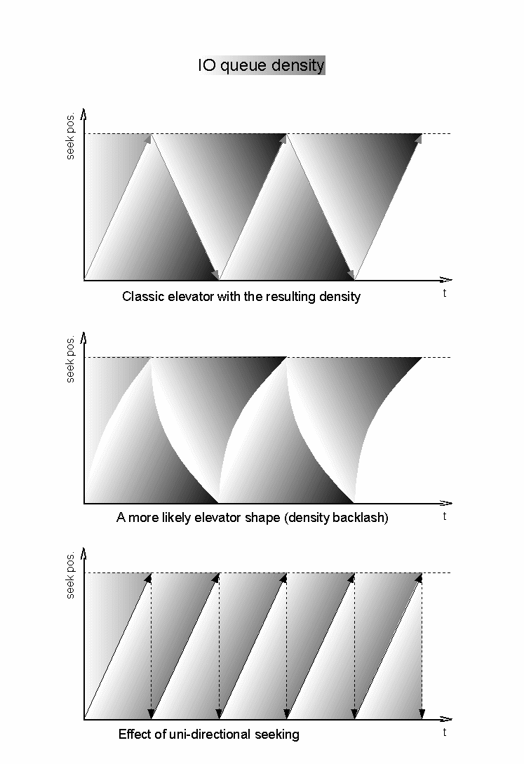
Which in turn makes me wonder, if the denser sections of the classic bi-directional elevator would mean performance improvement or degradation, and based on what metric :-) Total time of the sweep, MBps, IOps, or what... It would certainly depend on the level of randomness or OTOH write-combining made possible at the dense end of the queue...
Some say that the Solaris ZFS implementation is real good at squeezing the most out of the lazy spindles available, compared to Linux. ZFS seems to combine several layers, from VFS through LVM and some RAID features down to block-level interface against physical drives. This allows it to link bits of information among the different layers and act upon that knowledge efficiently. Maybe its scheduler solves some of the "circular reasoning" that I've presented above... without an excessive number of tuning knobs, it would seem.